This chapter gets you from nothing to a working simulation, then slows down and looks carefully at each piece. By the end you will know what every argument in the four-line pipeline does, what the table it produces looks like, and one subtle thing the four-line version gets slightly wrong, which turns out to be a preview of a real conservation law.
2.1 The Moon in four lines
library(orbitr)create_system() |>add_body("Earth", mass = mass_earth) |>add_body("Moon", mass = mass_moon, x = distance_earth_moon, vy = speed_moon) |>simulate_system(time_step = seconds_per_hour, duration = seconds_per_day *28) |>plot_orbits()
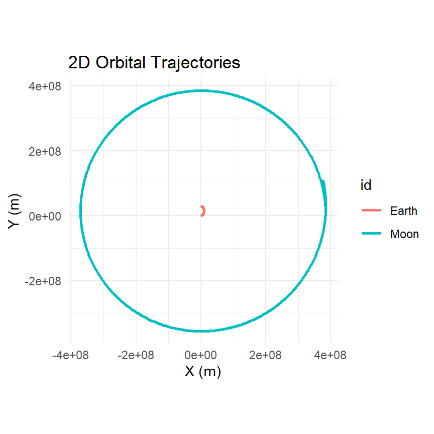
Figure 2.1: The Moon’s orbit around Earth over 28 days, simulated one hour at a time.
Earth sits at the origin. The Moon starts 384,400 km away along the \(x\) axis, moving at 1,022 m/s in the \(+y\) direction, and 28 days later it has gone around once. (The Earth’s own path is in there too; it is too small to see at this scale. We will come back to it.)
2.2 What each line does
create_system() makes an empty system. Its one argument is the gravitational constant, G, which defaults to the real value, \(6.6743\times10^{-11}\ \mathrm{m^3\,kg^{-1}\,s^{-2}}\). You will almost never change it, but it is there, and setting it to zero is a quick way to confirm that a body with no forces on it moves in a straight line.
add_body() adds one body. It needs a name (id) and a mass; everything else defaults to zero. The position arguments x, y, z are in meters and the velocity arguments vx, vy, vz in meters per second. Earth gets only a mass, so it starts at the origin at rest. The Moon gets a mass, an \(x\) position, and a \(y\) velocity. The constants mass_earth, mass_moon, distance_earth_moon, and speed_moon are exported by the package; Appendix D lists all of them with their sources.
simulate_system() runs the integration. time_step is the size of each step in seconds and duration is how long to run, also in seconds. Here that is one hour per step for 28 days, or \(28\times24 = 672\) steps. The defaults are one hour and one year. Two more arguments matter and have sensible defaults: method, which picks the integrator ("verlet" by default; Chapter 5), and softening, which is zero by default, meaning exact Newtonian gravity (Chapter 6).
plot_orbits() draws the path of every body with ggplot2 and returns the plot. Because it is an ordinary ggplot object you can add layers to it with +.
The constants seconds_per_hour, seconds_per_day, and seconds_per_year exist because every time argument in the package is in seconds, and nobody wants to type 2419200.
It is a tibble. Each row is one body at one instant. There are 1346 rows: two bodies, times 673 time steps, which is the 672 steps plus the initial state. The columns are the body’s id, its mass, its position x, y, z, its velocity vx, vy, vz, and time in seconds from the start.
That is the entire output format. There is nothing else to learn, which is the point: everything you already know how to do with a data frame works. How far is the Moon from the origin at the end of the run?
moon |>filter(time ==max(time)) |>mutate(r_km =sqrt(x^2+ y^2+ z^2) /1e3) |>select(id, time, r_km)#> # A tibble: 2 × 3#> id time r_km#> <chr> <dbl> <dbl>#> 1 Earth 2419200 29053.#> 2 Moon 2419200 391550.
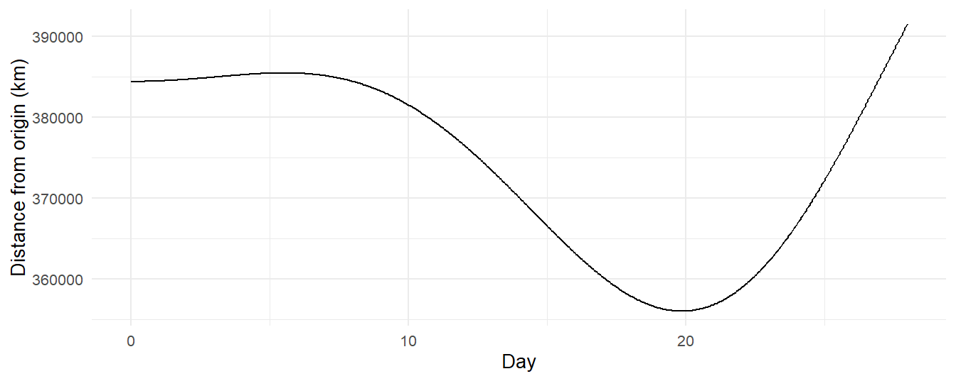
How does the Moon’s distance change over the month?
library(dplyr)library(ggplot2)moon |>filter(id =="Moon") |>mutate(r_km =sqrt(x^2+ y^2+ z^2) /1e3) |>ggplot(aes(time / seconds_per_day, r_km)) +geom_line() +labs(x ="Day", y ="Distance from origin (km)")
Figure 2.2: The Moon’s distance from the origin over the 28-day run. It is not quite constant: the orbit is slightly elliptical.
The distance dips and recovers: the orbit is an ellipse, not a circle, because 1,022 m/s is not exactly the speed that produces a circle at this distance. The speed that does is \(\sqrt{G(M+m)/r}\), which evaluates to
m/s. Chapter 4 derives that formula and shows how the small gap between it and 1,022 m/s determines the eccentricity of the orbit in Figure 2.2. For now, just notice that the simulation knows about it without being told.
2.4 Where did Earth go?
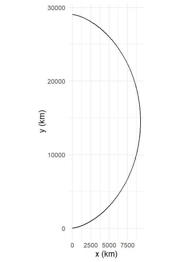
I said Earth’s path was too small to see. Let’s look at it on its own:
moon |>filter(id =="Earth") |>ggplot(aes(x /1e3, y /1e3)) +geom_path() +coord_equal() +labs(x ="x (km)", y ="y (km)")
Figure 2.3: Earth’s own motion during the 28-day run. It loops once around the pair’s center of mass while the whole system drifts in the \(+y\) direction.
Earth does not stay at the origin. It makes a small loop, as it should, because the Moon pulls on Earth just as Earth pulls on the Moon, and the two orbit their common center of mass. But the loop also drifts: after 28 days Earth has moved about
kilometers from where it started. Nothing is wrong with the simulation. The drift is the simulation being right about something we got wrong in the setup.
We gave the Moon momentum, \(m_{\mathrm{Moon}} \times 1022\ \mathrm{m/s}\) in the \(+y\) direction, and gave Earth none. The total momentum of the system is therefore not zero, and since gravity is an internal force, total momentum is conserved: the system’s center of mass has to keep moving at a constant velocity forever. That velocity is the Moon’s momentum divided by the total mass,
about 12 m/s, which over 28 days is 3.0027^{4} km. That is the drift in Figure 2.3, exactly.
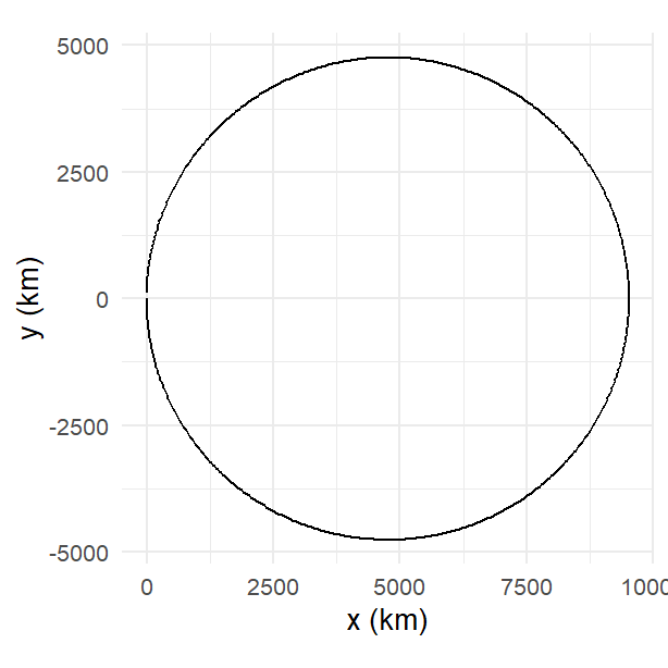
The fix is to give Earth the equal and opposite momentum so the total is zero. Earth’s velocity must be \(-v_{\mathrm{Moon}}\, m_{\mathrm{Moon}}/m_{\mathrm{Earth}}\):
v_earth <--speed_moon * mass_moon / mass_earthmoon_fixed <-create_system() |>add_body("Earth", mass = mass_earth, vy = v_earth) |>add_body("Moon", mass = mass_moon, x = distance_earth_moon, vy = speed_moon) |>simulate_system(time_step = seconds_per_hour, duration = seconds_per_day *28)moon_fixed |>filter(id =="Earth") |>ggplot(aes(x /1e3, y /1e3)) +geom_path() +coord_equal() +labs(x ="x (km)", y ="y (km)")
Figure 2.4: With zero total momentum, Earth’s path closes: a small circle around the center of mass, about 4,700 km from the origin.
Now Earth’s path closes. For a Sun-planet system the same drift exists and is a thousand times smaller, which is why the package’s add_sun() puts the Sun at rest at the origin and nobody notices. For a binary star, where the two masses are comparable, getting the momentum right is the whole problem, and Chapter 9 builds the Kepler-16 system from exactly this principle.
If you just want to look at the Moon going around Earth without thinking about the center of mass, there is a shortcut: re-center the data on Earth after the fact.
shift_reference_frame() subtracts Earth’s position and velocity from every body at every time step, which puts Earth at the origin for the whole run. And if what you want is the drift gone without re-running anything, shift_reference_frame(moon, "barycenter") re-centers every step on the pair’s center of mass, which is where the system was sitting all along. Chapter 10 is about what you can learn by doing this.
2.5 Real bodies without looking anything up
Typing masses, distances, and speeds works for any system you can imagine. For the real solar system there is an easier way. add_sun() places the Sun at the origin at rest, and add_planet() places a planet using its real orbital elements from the JPL DE440 ephemeris:
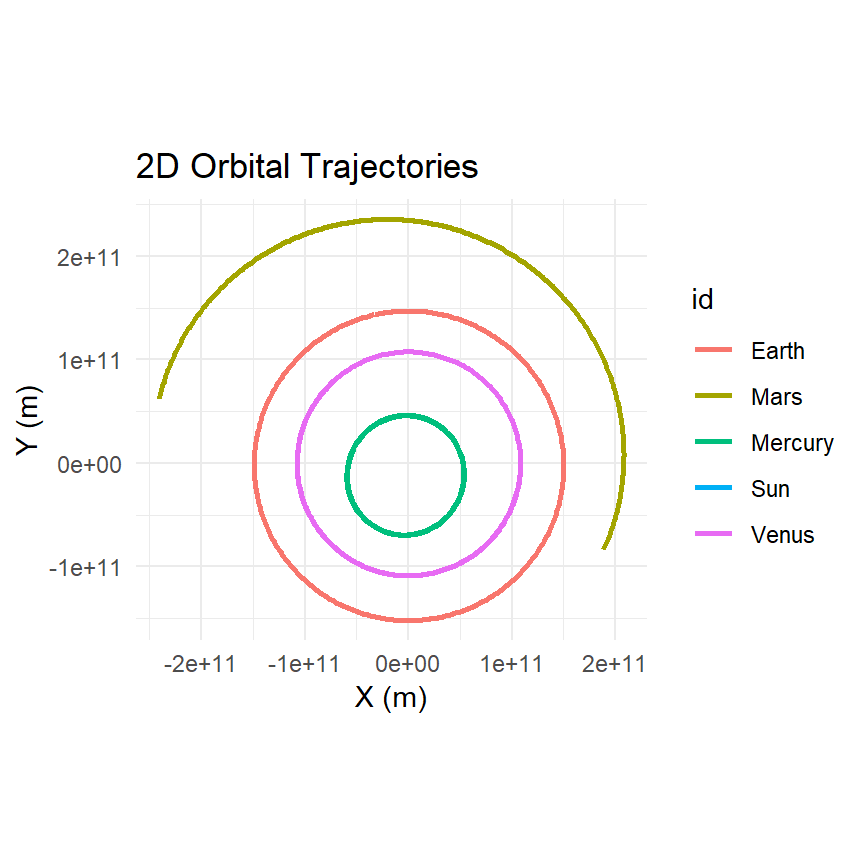
Figure 2.5: Mercury, Venus, Earth, and Mars for one Earth year, placed from JPL orbital elements.
parent = "Sun" tells add_planet() which body the orbit is around; the parent must already be in the system. Mercury completes about four orbits in the time Earth completes one, and you can see that its orbit is noticeably off-center: Mercury’s eccentricity is 0.21, the largest of any planet.
NoteWhy three_d = FALSE?
The real planets’ orbits are slightly tilted relative to one another, so once you use add_planet() the bodies have \(z\) motion. plot_orbits() notices and, by default, returns an interactive 3D plotly widget instead of a ggplot. That is the right thing on screen and the wrong thing on paper, so throughout this book I pass three_d = FALSE for any system with real orbital elements. On your own screen, leave it off and rotate the view.
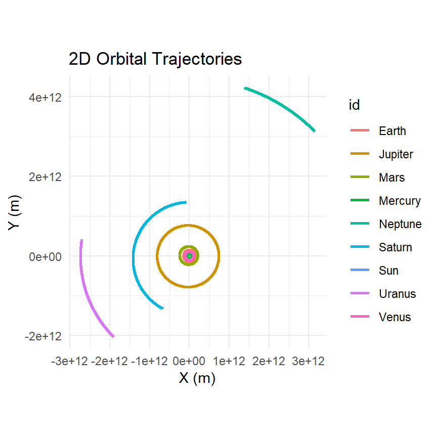
load_solar_system() builds the Sun, all eight planets, the Moon, and Pluto in one call, and remove_body() drops the ones you do not want:
Figure 2.6: The whole solar system for twelve years. The inner planets are a smudge at this scale; Neptune has completed less than a tenth of an orbit.
The Moon and Pluto are removed here for different reasons. Pluto’s orbit is large and does not change the picture. The Moon is removed because simulating it correctly needs a time step of an hour or so, and a twelve-year run at hourly steps is over a hundred thousand steps. One of the first things you learn about N-body simulation is that the time step is set by the fastest orbit in the system, not the one you care about. Chapter 5 explains why.
2.6 Looking before you leap
A system is an object you can inspect before you run it. Printing one shows the gravitational constant and the table of bodies:
sys <-create_system() |>add_sun() |>add_planet("Earth", parent ="Sun") |>add_planet("Mars", parent ="Sun")sys#> ───────────────────────────────── orbit_system ───────────────────────────────── #> G: 6.6743e-11 (standard)#> Bodies: 3#> #> # A tibble: 3 × 8#> id mass x y z vx vy vz#> <chr> <dbl> <dbl> <dbl> <dbl> <dbl> <dbl> <dbl>#> 1 Sun 1.99e30 0 0 0 0 0 0 #> 2 Earth 5.97e24 -32965585121. 143360295956. 0 -29520. -6788. 0 #> 3 Mars 6.42e23 188789951360. -83706961610. -6395443036. 10750. 24226. 243.
get_bodies() returns that table as a plain tibble, which is useful for checking that a hand-built system has the positions and velocities you intended:
get_bodies(sys) |>mutate(speed =sqrt(vx^2+ vy^2+ vz^2)) |>select(id, speed)#> # A tibble: 3 × 2#> id speed#> <chr> <dbl>#> 1 Sun 0 #> 2 Earth 30291.#> 3 Mars 26505.
Earth’s initial speed is a little over its mean orbital speed of 29,780 m/s, because add_planet() starts each body at periapsis (its closest approach to the Sun), where it moves fastest. The nu argument changes the starting point along the orbit; Chapter 7 covers it with the rest of the orbital elements.
2.7 Snapshots and animation
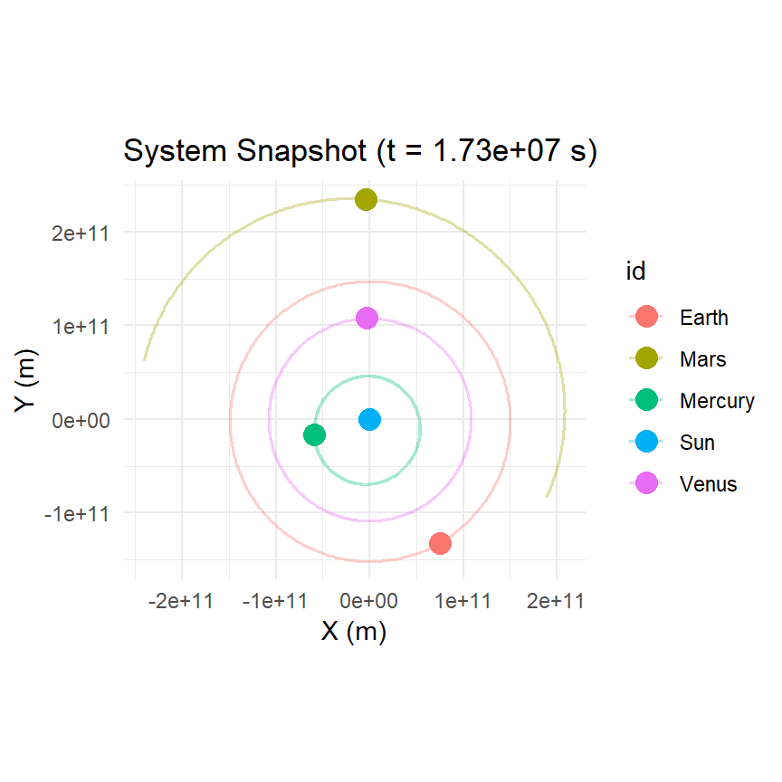
plot_orbits() draws whole trajectories. plot_system() draws where everything is at one instant, optionally with the trajectories drawn faintly behind:
Figure 2.7: The inner solar system at day 200 of the run, with trails.
The time argument is in simulation seconds and snaps to the nearest available step. A sequence of snapshots at different times is how the printed book shows motion. On screen, use the animation:
One Earth year of the inner solar system, animated (online edition).
This samples the run down to fps * duration frames and renders a GIF with gganimate (which you need to have installed, along with gifski). Each body leaves a fading wake. Rendering takes tens of seconds, so get the static plot right first.
2.8 Saving and sharing
save_system() writes a system, bodies and all, to an .rds file and load_system() reads it back, so a carefully tuned setup does not have to be rebuilt: